1.   Objective

Get acquainted with the data science ecosystem by exploring tabular data and using functions for sorting, ranking and plotting its content and thereby understanding a data collection content.

2.   Material

• Jupyter Notebook Server.
• Python Libraries.
• Data Collection: “csv”

3.   Importing necessary libraries

Let us begin by importing those toolboxes that we will need for our program. In the first cell we put the code to import the Pandas library as pd. This is for convenience; every time we need to use some functionality from the Pandas library, we will write pd instead of pandas. We will also import the two core libraries: the numpylibrary as np and the matplotliblibrary as plt.

import pandas as pd
import numpy as np
import matplotlib.pyplot as plt

Once the execution is finished, the header of the cell will be replaced by the next number of executions.

The DataFrameData Structure

The key data structure in Pandas is the DataFrameobject. A DataFrameis a tabular data structure, with rows and columns. Rows have a specific index to access them, which can be any name or value. In Pandas, the columns are called Series, a special type of data, which consists of a list of several values, where each value has an index.

Therefore, the DataFramedata structure can be seen as a spreadsheet, but it is much more flexible. To understand how it works, let us see how to create a DataFrame from a common Python dictionary of lists. First, we will create a new cell by clicking Insert Cell Belowor pressing the keys Ctrl + B. Then, we write in the following code:

data = {
'year': [2010, 2011, 2012,
2010, 2011, 2012,
2010, 2011, 2012],
'team': ['FCBarcelona', 'FCBarcelona', 'FCBarcelona',
'RMadrid', 'RMadrid', 'RMadrid',
'ValenciaCF', 'ValenciaCF', 'ValenciaCF'],
'wins': [30, 28, 32, 29, 32, 26, 21, 17, 19],
'draws': [6, 7, 4, 5, 4, 7, 8, 10, 8],
'losses': [2, 3, 2, 4, 2, 5, 9, 11, 11]
}

football = pd.DataFrame(data, columns = ['year', 'team', 'wins', 'draws', 'losses'])

In this example, we use the pandas DataFrameobject constructor with a dictionary of lists as argument. The value of each entry in the dictionary is the name of the column, and the lists are their values.

The DataFrame columns can be arranged at construction time by entering a key- word columns with a list of the names of the columns ordered as we want. If the column keyword is not present in the constructor, the columns will be arranged in alphabetical order. Each entry in the dictionary is a column. The index of each row is created automatically taking the position of its elements inside the entry lists, starting from 0.

5.   To Do and To Hand In

• Go through the exercise and execute the functions that help you explore the content of the data collection.
• Add markdown cells in your Kaggle notebook comment your results and answer the questions stated in blue within the exercice (include the question in your markdown cell). 
• Download your notebook. Share it in your personal shared folder (as previous material) and share the link here (column HO-1).

6.   Playing with the Education and training data

This exercise us based on a Eurostat data collection, used to process and publish comparable statistical information at the European level. The data in Eurostat are provided by each member state and it is free to reuse them, for both noncommercial and commercial purposes (with some minor exceptions).

Since the amount of data in the Eurostat database is huge, in our first study we only focus on data relative to indicators of educational funding by the member states. Thus, the first thing to do is to retrieve such data from Eurostat. Since open data have to be delivered in a plain text format, CSV (or any other delimiter-separated value) formats are used to store tabular data. In a delimiter-separated value file, each line is a data record and each record consists in one or more fields, separated by the delimiter character (usually a comma). The data collection used in this exercise can be found already processed at the Data Science book’s Github repository as educ_figdp_1_Data.csvfile.

6.1  Reading data

Let us start reading the educ_figdp_1_Data.csv file stored in the same directoryas your notebook directory. Write the following code to read and show the content:

edu = pd.read_csv('files/ch02/educ_figdp_1_Data.csv',
                  na_values=':', usecols=['TIME', 'GEO', 'Value'])
edu

The way to read CSV (or any other separated value, providing the separator character) files in Pandas is by calling the method read_csv. Besides the name of the file, we add the key argument na_valuesto this method along with the character that represents “non available data” in the file.

Normally, CSV files have a header with the names of the columns. If this is the case, we can use the usecolsparameter to select which columns in the file will be used.

In this case, the DataFrameresulting from reading our data is stored in edu.

1. Which is the size of the edu DataFrame (rows x columns)?

Since the DataFrameis too large to be fully displayed, three dots appear in the middle of each row.

To see how the data looks, we can use the method head(), which shows just the first five rows.

2. What happens if we give a number as argument to the method head()?

edu.head()

Similarly, it exists the method tail().

3. What does the method tail()return?

edu.tail()

If we want to know the names of the columns or the names of the indexes, we can use the DataFrameattributes columnsand indexrespectively. The names of the columns or indexes can be changed by assigning a new list of the same length to these attributes. The values of any DataFramecan be retrieved as a Python array by calling its values attribute.

If we just want quick statistical information on all the numeric columns in a DataFrame, we can use the function describe().

4. Which measures does the result show? It seems that it shows some default values, can you guess which ones?

edu.describe()

6.2  Selecting data

If we want to select a subset of data from a DataFrame, it is necessary to indicate this subset using square brackets ([ ])after the DataFrame. The subset can be specified in several ways. If we want to select only one column from a DataFrame, we only need to put its name between the square brackets. The result will be a Seriesdata structure, not a DataFrame, because only one column is retrieved.

edu['Value']

If we want to select a subset of rows from a DataFrame, we can do so by indicating a range of rows separated by a colon (:) inside the square brackets. This is known as a slice of rows:

edu[10:14]

This instruction returns the slice of rows from the 10th to the 13th position. Note that the slice does not use the index labels as references, but the position. In this case, the labels of the rows simply coincide with the position of the rows.

If we want to select a subset of columns and rows using the labels as our references instead of the positions, we can use ilocindexing:

edu.loc[90:94][['TIME','GEO']]

5. What does this index return? What does the first index represent? And the second one?

6.3  Filtering data

Another way to select a subset of data is by applying Boolean indexing. This indexing is known as a filter. For instance, if we want to filter those values less than or equal to 6.5, we can do it like this:

edu[edu['Value'] > 6.5].tail()

Boolean indexing uses the result of a Boolean operation over the data, returning a mask with True or False for each row. The rows marked True in the mask will be selected.

6. What does the operation edu[’Value’] > 6.5 produce? An if we apply the indexedu[edu[’Value’] > 6.5]?Is this aSeries or aDataFrame?

Of course, any of the usual Boolean operators can be used for filtering: < (less than),<= (less than or equal to), > (greater than), >= (greater than or equal to), == (equal to), and ! = (not equal to).

6.4  Filtering missing values

Pandas uses the special value NaN(not a number) to represent missing values. In Python, NaNis a special floating-point value returned by certain operations when one of their results ends in an undefined value. A subtle feature ofNaNvalues is that two NaNare never equal. Because of this, the only safe way to tell whether a value is missing in a DataFrameis by using the function isnull(). Indeed, this function can be used to filter rows with missing values:

edu[edu["Value"].isnull()].head()

6.5  Manipulating data

Once we know how to select the desired data, the next thing we need to know is how to manipulate data. One of the most straightforward things we can do is to operate with columns or rows using aggregation functions.

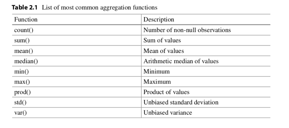
Table 2.1 shows a list of the most common aggregation functions. The result of all these functions applied to a row or column is always a number. Meanwhile, if a function is applied to a DataFrameor a selection of rows and columns, then you can specify if the function should be applied to the rows for each column (setting the axis=0 keyword on the invocation of the function), or it should be applied on the columns for each row (setting the axis=1 keyword on the invocation of the function).

edu.max(axis = 0)

Note that these are functions specific to Pandas, not the generic Python functions. There are differences in their implementation. In Python, NaNvalues propagate through all operations without raising an exception. In contrast, Pandas operations exclude NaNvalues representing missing data. For example, the Pandas maxfunction excludes NaNvalues, thus they are interpreted as missing values, while the standard Python max function will take the mathematical interpretation of NaNand return it as the maximum:

print ('Pandas max function:', edu['Value'].max())
print ('Python max function:', max(edu['Value']))

Beside these aggregation functions, we can apply operations over all the values in rows, columns or a selection of both. The rule of thumb is that an operation between columns means that it is applied to each row in that column and an operation between rows means that it is applied to each column in that row. For example we can apply any binary arithmetical operation (+,-,*,/) to an entire row:

s = edu["Value"]/100
s.head()

However, we can apply any function to a DataFrameor Seriesjust setting its name as argument of the apply method. For example, in the following code, we apply the sqrt function from the NumPylibrary to perform the square root of each value in the column Value.

s = edu["Value"].apply(np.sqrt)
s.head()

If we need to design a specific function to apply it, we can write an in-line function, known as a λ-function. A λ-function is a function without a name. It is only necessary to specify the parameters it receives, between the lambda keyword and the colon (:). In the next example, only one parameter is needed, which will be the value of each element in the column Value. The value the function returns will be the square of that value.

s = edu["Value"].apply(lambda d: d**2)
s.head()

Another basic manipulation operation is to set new values in our DataFrame. This can be done directly using the assign operator (=) over a DataFrame. For example, to add a new column to a DataFrame, we can assign a Seriesto a selection of a column that does not exist.

This will produce a new column in the DataFrameafter all the others. You must be aware that if a column with the same name already exists, the previous values will be overwritten. In the following example, we assign the Seriesthat results from dividing the columnValueby the maximum value in the same column to a new column named ValueNorm.

edu['ValueNorm'] = edu['Value']/edu['Value'].max()
edu.tail()

Now, if we want to remove this column from the DataFrame, we can use the function drop.

This removes the indicated rows if axis=0, or the indicated columns if axis=1.

In Pandas, all the functions that change the contents of a DataFrame, such as the function drop, will normally return a copy of the modified data, instead of overwriting the DataFrame. Therefore, the original DataFrameis kept. If you do not want to keep the old values, you can set the keyword inplaceto True. By default, this keyword is set toFalse, meaning that a copy of the data is returned.

edu.drop('ValueNorm', axis = 1, inplace = True)
edu.head()

Instead, if what we want to do is to insert a new row at the bottom of the DataFrame, we can use the Pandas function append. This function receives as argument the new row, which is represented as a dictionary where the keys are the name of the columns and the values are the associated value. You must be aware to setting the ignore_indexflag in the append method to True, otherwise the index 0 is given to this new row, which will produce an error if it already exists:

edu = edu.append({"TIME": 2000, "Value": 5.00, "GEO": 'a'},
                  ignore_index = True)
edu.tail()

Finally, if we want to remove this row, we need to use the function dropagain. Now we have to set the axis to 0, and specify the index of the row we want to remove. Since we want to remove the last row, we can use the max function over the indexes to determine which row is.

edu.drop(max(edu.index), axis = 0, inplace = True)
edu.tail()

The function isnull()can be used to remove NaN values. This has a similar effect to filtering the NaN values, as explained above, but here the difference is that a copy of the DataFramewithout the NaNvalues is returned, instead of a view.

eduDrop = edu[~edu["Value"].isnull()].copy()
eduDrop.head()

To remove NaNvalues, instead of the generic functiondrop, we can use the specific function dropna(). If we want to erase any row that contains an NaN value, we have to set the how keyword to any. To restrict it to a subset of columns, we can specify it using the subset keyword. As we can see below, the result will be the same as using the function drop:

eduDrop = edu.dropna(how = 'any', subset = ["Value"])
eduDrop.head()

If, instead of removing the rows containing NaN, we want to fill them with another value, then we can use the method fillna(), specifying which value has to be used. If we want to fill only some specific columns, we have to set as argument to the function fillna()a dictionary with the name of the columns as the key and which character to be used for filling as the value.

eduFilled = edu.fillna(value = {"Value": 0})
eduFilled.head()

6.6  Sorting data

Another important functionality we will need when inspecting our data is to sort by columns. We can sort a DataFrameusing any column, using the sort function. If we want to see the first five rows of data sorted in descending order (i.e., from the largest to the smallest values) and using the column Value, then we just need to do this:

edu.sort_values(by = 'Value', ascending = False,
                inplace = True)
edu.head()

Note that the keyword inplacemeans that the DataFramewill be overwritten, and hence no new DataFrameis returned. If instead of ascending = Falsewe use ascending = True, the values are sorted in ascending order (i.e., from the smallest to the largest values).

If we want to return to the original order, we can sort by an index using the function sort_indexand specifying axis=0:

edu.sort_index(axis = 0, ascending = True, inplace = True)
edu.head()

6.7  Grouping data

Another very useful way to inspect data is to group it according to some criteria. For instance, in our example it would be nice to group all the data by country, regardless of the year.

Pandas has the function groupbythat allows us to do exactly this. The value returned by this function is a special grouped DataFrame. To have a proper DataFrameas a result, it is necessary to apply an aggregation function. Thus, this function will be applied to all the values in the same group.

For example, in our case, if we want a DataFrameshowing the mean of the values for each country over all the years, we can obtain it by grouping according to country and using the function meanas the aggregation method for each group. The result would be a DataFramewith countries as indexes and the mean values as the column:

group = edu[["GEO", "Value"]].groupby('GEO').mean()
group.head()

6.8  Rearranging data

Up until now, our indexes have been just a numeration of rows without much meaning. We can transform the arrangement of our data, redistributing the indexes and columns for better manipulation of our data, which normally leads to better performance. We can rearrange our data using the function pivot_table. Here, we can specify which columns will be the new indexes, the new values, and the new columns.

For example, imagine that we want to transform our DataFrameto a spreadsheet- like structure with the country names as the index, while the columns will be the years starting from 2006 and the values will be the previous Value column.

To do this, first we need to filter out the data and then pivot it in this way:

filtered_data = edu[edu["TIME"] > 2005]
pivedu = pd.pivot_table(filtered_data, values = 'Value',
                        index = ['GEO'], columns = ['TIME'])
pivedu.head()

Now we can use the new index to select specific rows by label, using the locoperator:

pivedu.loc[['Spain','Portugal'], [2006,2011]]

Pivot also offers the option of providing an argument aggr_functionthat allows to perform an aggregation function between the values if there is more than one value for the given row and column after the transformation. As usual, you can design any custom function you want, just giving its name or using a λ-function.

6.9  Ranking data

Another useful visualization feature is to rank data. For example, we would like to know how each country is ranked by year.

To see this, we will use the Pandas functionrank. But first, we need to clean up our previous pivoted table a bit so that it only has real countries with real data. To do this, first we drop the Euro area entries and shorten the Germany name entry, using the rename function and then we drop all the rows containing any NaN, using the function dropna.

Now we can perform the ranking using the function rank.

7. What do you observe regarding the parameter ascending=False?

The Pandas function ranksupports different tie-breaking methods, specified with the method parameter. In our case, we use the first method, in which ranks are assigned in the order they appear in the array, avoiding gaps between ranking.

pivedu = pivedu.drop(['Euro area (13 countries)',
                      'Euro area (15 countries)',
                      'Euro area (17 countries)',
                      'Euro area (18 countries)',
                      'European Union (25 countries)',
                      'European Union (27 countries)',
                      'European Union (28 countries)'
                      ], axis=0)
pivedu = pivedu.rename(
    index={'Germany (until 1990 former territory of the FRG)': 'Germany'})
pivedu = pivedu.dropna()
pivedu.rank(ascending=False, method='first').head()

If we want to make a global ranking considering all the years, we can sum up all the columns and rank the result. Then we can sort the resulting values to retrieve the top five countries for the last 6 years, in this way:

totalSum = pivedu.sum(axis = 1)

totalSum.rank(ascending = False, method = 'dense').sort_values().head()

Note that the method keyword argument in the in the function rankspecifies how items that compare equals receive ranking. In the case of dense, items that compare equals receive the same ranking number, and the next not equal item receives the immediately following ranking number.

7.1  Plotting data

Pandas DataFramesand Seriescan be plotted using the function plot, which uses the library for graphics Matplotlib. For example, if we want to plot the accumulated values for each country over the last 6 years, we can take the Seriesobtained in the previous example and plot it directly by calling the plot function as shown in the next cell:

totalSum = pivedu.sum(axis = 1).sort_values(ascending = False)
totalSum.plot(kind = 'bar', style = 'b', alpha = 0.4,
              title = "Total Values for Country")

Note that if we want the bars ordered from the highest to the lowest value, we need to sort the values in theSeriesfirst. The parameter kind used in the function plotdefines which kind of graphic will be used.

In our case, a bar graph. The parameter style refers to the style properties of the graphic, in our case, the color of bars is set to b (blue). The alpha channel can be modified adding a keyword parameter alpha with a percentage, producing a more translucent plot. Finally, using the title keyword the name of the graphic can be set.

It is also possible to plot a DataFramedirectly. In this case, each column is treated as a separated Series. For example, instead of printing the accumulated value over the years, we can plot the value for each year.

my_colors = ['b', 'r', 'g', 'y', 'm', 'c']
ax = pivedu.plot(kind='barh', stacked=True, color=my_colors, figsize=(12, 6))
ax.legend(loc='center left', bbox_to_anchor=(1, 0.5))
plt.savefig('Value_Time_Country.png', dpi=300, bbox_inches='tight')

In this case, we have used a horizontal bar graph (kind=’barh’) stacking all the years in the same country bar. This can be done by setting the parameter stackedto True.

The number of default colors in a plot is only 5, thus if you have more than 5 Series to show, you need to specify more colors or otherwise the same set of colors will be used again. We can set a new set of colors using the keyword colorwith a list of colors.

Basic colors have a single-character code assigned to each, for example, “b” is for blue, “r” for red, “g” for green, “y” for yellow, “m” for magenta, and “c” for cyan. When several Series are shown in a plot, a legend is created for identifying each one. The name for each Series is the name of the column in the DataFrame. By default, the legend goes inside the plot area.

If we want to change this, we can use the legend function of the axis object (this is the object returned when the plot function is called). By using the keyword loc, we can set the relative position of the legend with respect to the plot. It can be a combination of right or left and upper, lower, or center. With bbox_to_anchor we can set an absolute position with respect to the plot, allowing to put the legend outside the graph.

Appendix: Launching the platform

A.1 Manually

• Open a terminal and type $jupyter notebook

A.2 Click & run

If you chose the bundle installation, you can start the Jupyter notebook platform by clicking on the Jupyter Notebook icon installed by Anaconda in the start menu or on the desktop.

The browser will immediately be launched displaying the Jupyter notebook home- page, whose URL is http://localhost:8888/tree. Note that a special port is used by default it is 8888.

This initial page displays a tree view of a directory.

• If you use the command line, the root directoryis the same directory where you launched the Jupyter notebook.
• Otherwise, if you use the Anaconda launcher, the root directoryis the current user directory.

Now, to start a new notebook, we only need to press the button

New --> Notebooks -->Python 2

at the top on the right of the home page.

Click on the notebook name and rename it for example like Open Government Data Analysis.