The objective of this exercise is to show you how to create a map using D3.js and TopoJSON, a lighter version of GeoJSON.
Requirements
- Node
- Geospatial Data Abstraction Library (GDAL)
- Natural Earth data (provided during the course)
- JQ JSON processor
- TopoJSON (v. 1x) & http-server (node packages)
Obtaining and preparing the data
The first step for creating a map is to obtain earth data. A great resource for this is Natural Earth. In this exercise, we will create a map of United Kingdom using the following Natural Earth datasets:
- Admin 0 – Details – map subunits (scale 1:10m)
- Populated Places (scale 1:10m)
The former contains polygons representing subdivisions of 197 countries; the latter names and locations of populated places.
For simplicity, we are providing both datasets as part of the exercise material.
The Natural Earth datasets contain several files which are not adapted for the web. The most important of these files is called shapefile (‘.shp’). Thus, the next step consists in transforming the shapefiles (‘.shp’) into GeoJSON as follows:
ogr2ogr \
   -f GeoJSON \
   -where "ADM0_A3 IN ('GBR', 'IRL')" \
   subunits.json \
  data/map_subunits/ne_10m_admin_0_map_subunits.shp
This instruction uses the ogr2ogr tool of the GDAL library and creates a file called subunits.json containing only the polygons of UK and Ireland. The filter is done by passing a conditional SQL expression in —where option. In the filter expression, ADM0 refers to Admin-0, the highest level administrative boundaries, and A3 refers to ISO 3166-1 alpha-3 country codes. Although the objective of the exercise is to map only the United Kingdom, we need the information about Ireland to portray land accurately. Otherwise, we would give the impression that Northern Ireland is an island.
The subunits.json file contains more information than the polygons delimitating UK and Ireland. You can see this by navigating through the GeoJSON object contained in the file:
jq '.features[0].properties' subunits.json
This instruction projects the attributes associated to a country subdivision (i.e., subunit) using JQ query expression.
The JQ has a lot of nice features. For instance, the following example collects all the attributes (keys) of the objects contained in the GeoJSON object:
jq ‘.. | objects | keys[]’ subunits.json
See the manual for more information.
The map we are creating will include the names of the main cities of United Kingdom. This information is contained in the ne_10m_populated_places.shp. Thus, the next step consists in transforming and filtering the populated places file keeping only the information related to UK.
ogr2ogr \
  -f GeoJSON \
  -where "ISO_A2 = 'GB' AND SCALERANK < 8" \
  places.json \
  data/populated_places/ne_10m_populated_places.shp
The places’ properties are (somewhat arbitrarily) different, so the where clause of this instructions refers to ISO_A2 instead of ADM0_A3. The SCALERANK filter further whittles the labels down to major cities.
File reduction
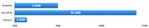
GeoJSON files are usually too big for the web because they contain a lot of redundant information. TopoJSON in contrast, an extension of GeoJSON, only contains information about the topology, reducing the file size up to 80% (see figure below).
The following instruction shows you how to transform a GeoJSON file into TopoJSON:
topojson \
  -o uk.json \
  --id-property SU_A3 \
  --properties name=NAME \
  -- \
  subunits.json \
  places.json
This instruction combine the subunits.json and places.json files into a single one called uk.json. This step includes a minor transformation to fix the inconsistencies in the datasets, renaming the NAME property to name, and promoting the SU_A3 property to the object id. You can see the resulting ids as follows:
jq '.objects.subunits.geometries[].id' uk.json
You can also see confirm the storage space occupied by each of the GeoJSON and TopoJSON files as follows:
ls -lh *.json
Creating the Web Page
Once you have the data ready you can start plotting the map. For this, you will start with the index.html file which contains the following code:
<!DOCTYPE html>
<meta charset="utf-8">
<style>
/* CSS goes here. */
</style>
<body>
Simple UK map
<script src="lib/d3.v3.min.js" charset="utf-8"></script>
<script src="lib/topojson.v1.min.js"></script>
<script>
/* JavaScript goes here. */
</script>
Start local web server to view the web page.
http-server -p 8008
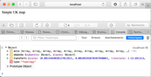
When you load this html file (http://localhost:8008) you will only get the string “Simple UK map”. For loading the data into the map replace the /* JavaScript goes here. */ part with the following code:
d3.json("uk.json", function(error, uk) {
   if (error) return console.error(error);
   console.log(uk);
 });
Now, if you peek at your JavaScript console, you should see a topology object containing the boundaries of UK’ subdivisions.
Displaying polygons
There are a variety of ways to render two-dimensional geometry in a browser, but the two main standards are SVG and Canvas. D3 3.0 supports both. For this exercise, we will use SVG because it can be easily styled via CSS.
To create the root SVG element copy/paste the following code into the script:
var width = 960,
    height = 1160;

var svg = d3.select("body").append("svg")
    .attr("width", width)
    .attr("height", height);
The recommended place to put this code is at the top of the script rather than inside the d3.json callback. That is because d3.json is asynchronous (i.e., the rest of the page will render while the TopoJSON file is downloaded). Creating the empty SVG root when the page first loads avoids distracting reflow when the geometry finally arrives.
There are 2 more things required for rendering a geography: a projection and a path generator.
The projection maps spherical coordinate to the Cartesian plane, which is required to display spherical geometry on a 2D screen (you can skip this if this is the future and you’re using a 3D holographic display); the path generator takes the projected 2D geometry and formats it appropriately for SVG or Canvas.
For creating a map replace the code inside the d3.json callback like so:
d3.json("uk.json", function(error, uk) {
  if (error) return console.error(error);
  svg.append("path")
      .datum(topojson.feature(uk, uk.objects.subunits))
      .attr("d", d3.geo.path().projection(d3.geo.mercator()));
});
You should now see a small, black and familiar speck:

Recall from earlier the two closely-related JSON geographic data formats: GeoJSON and TopoJSON. While our data can be stored more efficiently in TopoJSON, we must convert back to GeoJSON for display. Lets break this step out to make it explicit:
var subunits = topojson.feature(uk, uk.objects.subunits);
Similarly, we can extract the definition of the projection to make the code clearer:
 var projection = d3.geo.mercator()
    .scale(500)
    .translate([width / 2, height / 2]);
And likewise, the path generator:
var path = d3.geo.path()
    .projection(projection);
And the path element, to which we bind the GeoJSON data, and then use selection.attr to set the “d” attribute to the formatted path data:
svg.append("path")
    .datum(subunits)
    .attr("d", path);
With the code structured like this, we can now change the projection to something more suitable for the United Kingdom. The Albers equal-area conic projection is a good choice, with standard parallels of 50°N and 60°N. To position the map, we rotate longitude by +4.4° and set the center to 0°W 55.4°N, giving an effective origin of 4.4°W 55.4°N, somewhere in a field in Scotland.
var projection = d3.geo.albers()
    .center([0, 55.4])
    .rotate([4.4, 0])
    .parallels([50, 60])
    .scale(6000)
    .translate([width / 2, height / 2]);
Your map should now look much better.
Styling Polygons
As mentioned before, a benefit of SVG is that it can be stylized with CSS. In what follows, you will add color to countries’ subdivisions using style rules that assign a value to the fill property. However, you must give first each country its own path element rather than sharing one. Without distinct path elements, we have no way to assign distinct colors.
Within the uk.json TopoJSON file, the Admin-0 map subunits are represented as a feature collection. By pulling out the features array, we can compute a data join and create a path element for each feature:
//replace previous svg.append with this code
svg.selectAll(".subunit")
  .data(subunits.features)
  .enter().append("path")
    .attr("class", function(d) { return "subunit " + d.id; })
    .attr("d", path);
We can also compute the “class” attribute as a function of data, so that in addition to the subunit class, each country has a three-letter class corresponding to its ISO-3166 alpha-3 country code. These allow us to apply separate fill styles for each country:
.subunit.SCT { fill: #ddc; }
.subunit.WLS { fill: #cdd; }
.subunit.NIR { fill: #cdc; }
.subunit.ENG { fill: #dcd; }
.subunit.SCT { fill: #ddc; }
.subunit.IRL { display: none; }
Displaying Boundaries
To apply the finishing touch to the polygons, we need a few lines. These are two boundary lines representing the borders of England with Scotland and Wales, respectively, and the Irish coastline.
We’ll use topojson.mesh to compute the boundaries from the topology. This requires two arguments: the topology and a constituent geometry object. An optional filter can reduce the set of returned boundaries, taking two arguments a and b representing the two features on either side of the boundary. For exterior boundaries such as coastlines, a and b are the same. Thus by filtering on a === b or a !== b, we obtain exterior or interior boundaries exclusively.
svg.append("path")
    .datum(topojson.mesh(uk, uk.objects.subunits, function(a, b) { return a !== b && a.id !== "IRL"; }))
    .attr("d", path)
    .attr("class", "subunit-boundary");
That leaves only the Irish coastline, an exterior boundary:
svg.append("path")
    .datum(topojson.mesh(uk, uk.objects.subunits, function(a, b) { return a === b && a.id === "IRL"; }))
    .attr("d", path)
    .attr("class", "subunit-boundary IRL");
Add a bit of style:
.subunit-boundary {
  fill: none;
  stroke: #777;
  stroke-dasharray: 2,2;
  stroke-linejoin: round;
}

.subunit-boundary.IRL {
  stroke: #aaa;
}
And voilà!
Displaying Places
As with the country polygons, the populated places are a feature collection, so we can again convert from TopoJSON to GeoJSON and use d3.geo.path to render:
svg.append("path")
    .datum(topojson.feature(uk, uk.objects.places))
    .attr("d", path)
    .attr("class", "place");
This will draw a small circle for each city. We can adjust the radius by setting path.pointRadius, and assign styles via CSS.
text {
 font-family: "Helvetica Neue", Helvetica, Arial, sans-serif;
 font-size: 10px;
 pointer-events: none;
}
We also want labels, so we need a data join to create text elements. By computing the transform property by projecting the place’s coordinates, we translate the labels into the desired position:
svg.selectAll(".place-label")
    .data(topojson.feature(uk, uk.objects.places).features)
  .enter().append("text")
    .attr("class", "place-label")
    .attr("transform", function(d) { return "translate(" + projection(d.geometry.coordinates) + ")"; })
    .attr("dy", ".35em")
    .text(function(d) { return d.properties.name; });
Labeling a map well can be challenging, especially if you want to position labels automatically. We’ve mostly ignored the problem for our simple map, though it helps that we earlier filtered labels by SCALERANK. A convenient trick is to use right-aligned labels on the left side of the map, and left-aligned labels on the right side of the map, here using 1°W as the threshold:
svg.selectAll(".place-label")
    .attr("x", function(d) { return d.geometry.coordinates[0] > -1 ? 6 : -6; })
    .style("text-anchor", function(d) { return d.geometry.coordinates[0] > -1 ? "start" : "end"; });
Country Labels
Our map is missing a critical component: we haven’t labeled the countries! We could have used Natural Earth’s Admin-0 label points, but we can just as easily compute country label points using the projected centroid:
svg.selectAll(".subunit-label")
    .data(topojson.feature(uk, uk.objects.subunits).features)
  .enter().append("text")
    .attr("class", function(d) { return "subunit-label " + d.id; })
    .attr("transform", function(d) { return "translate(" + path.centroid(d) + ")"; })
    .attr("dy", ".35em")
    .text(function(d) { return d.properties.name; });
The country labels are styled larger to distinguish them from city labels. By making them partly transparent, country labels are relegated to the background and city labels are more legible:
.subunit-label {
  fill: #777;
  fill-opacity: .5;
  font-size: 20px;
  font-weight: 300;
  text-anchor: middle;
}
And there we have it.